Subsections

• 11.3.1 Preamble: Monte Carlo Importance Sampling
• 11.3.2 First Illustrations
• 11.3.3 Approximations of the Bayes Factor

11.3 Monte Carlo Methods

The natural approach to these computational problems is to use computer simulation and Monte Carlo techniques, rather than numerical methods, simply because there is much more to gain from exploiting the probabilistic properties of the integrands rather than their analytical properties. In addition, the dimension of most problems considered in current Bayesian Statistics is such that very involved numerical methods should be used to provide a satisfactory approximation in such integration or optimisation problems. Indeed, down-the-shelf numerical methods cannot handle integrals in dimensions larger than $4$ and more advanced numerical integration methods require analytical studies on the distribution of interest.

11.3.1 Preamble: Monte Carlo Importance Sampling

Given the statistical nature of the problem, the approximation of an integral like

$$\mathfrak{I} = \int_{\Theta} h(\theta) f(x\vert\theta) \pi(\theta) \,{\text{d}}\theta\;,$$

should indeed take advantage of the special nature of $\mathfrak{I}$, namely, the fact that $\pi$ is a probability density^11.4 or, instead, that $f(x\vert\theta) \pi(\theta)$ is proportional to a density. As detailed in Chap. II.2 this volume, or in Robert and Casella (2004, Chap. 3), the Monte Carlo method was introduced by [30] and [44] for this purpose. For instance, if it is possible to generate (via a computer) random variables $\theta_1, \ldots,\theta_m$ from $\pi(\theta)$, the average

$$\frac{1}{ m}\sum_{i=1}^m h(\theta_i) f(x\vert\theta_i)$$

converges (almost surely) to $\mathfrak{I}$ when $m$ goes to $+\infty$, according to the Law of Large Numbers. Obviously, if an i.i.d. sample of $\theta _i$'s from the posterior distribution $\pi(\theta\vert x)$ can be produced, the average

$$\frac{1}{ m}\sum_{i=1}^m h(\theta_i)$$ (11.4)

converges to

$$\mathbb{E}^{\pi} [h(\theta)\vert x] = \frac{\int_{\Theta} h(\thet... ...\text{d}}\theta} {\int_{\Theta} f(x\vert\theta) \pi(\theta) \,{\text{d}}\theta}$$

and it usually is more interesting to use this approximation, rather than

$$\sum_{i=1}^m h(\theta_i) f(x\vert\theta_i) \bigg/ \sum_{i=1}^m f(x\vert\theta_i)$$

when the $\theta _i$'s are generated from $\pi(\theta)$, especially when $\pi(\theta)$ is flat compared with $\pi(\theta\vert x)$.

In addition, if the posterior variance var$(h(\theta)\vert x)$ is finite, the Central Limit Theorem applies to the empirical average (11.4), which is then asymptotically normal with variance var$(h(\theta)\vert x)/m$. Confidence regions can then be built from this normal approximation and, most importantly, the magnitude of the error remains of order $1/\sqrt m$, whatever the dimension of the problem, in opposition with numerical methods.^11.5 (See also [37], Chap. 4, for more details on the convergence assessment based on the CLT.)

The Monte Carlo method actually applies in a much wider generality than the above simulation from $\pi$. For instance, because $\mathfrak{I}$ can be represented in an infinity of ways as an expectation, there is no need to simulate from the distributions $\pi(\cdot\vert x)$ or $\pi$ to get a good approximation of  $\mathfrak{I}$. Indeed, if $g$ is a probability density with supp$(g)$ including the support of $\vert h(\theta)\vert f(x\vert\theta) \pi(\theta)$, the integral $\mathfrak{I}$ can also be represented as an expectation against $g$, namely

$$\int \frac{h(\theta) f(x\vert\theta) \pi(\theta)}{g(\theta)} g(\theta) \,{\text{d}}\theta\;.$$

This representation leads to the Monte Carlo method with importance function $g$: generate $\theta_1, \ldots,\theta_m$ according to $g$ and approximate $\mathfrak{I}$ through

$$\frac{1}{ m} \sum_{i=1}^m h(\theta_i) \omega_i(\theta_i)\;,$$

with the weights $\omega(\theta_i)=f(x\vert\theta_i)\pi(\theta_i)/g(\theta_i)$. Again, by the Law of Large Numbers, this approximation almost surely converges to  $\mathfrak{I}$. And this estimator is unbiased. In addition, an approximation to $\mathbb{E}^{\pi}[h(\theta)\vert x]$ is given by

$$\frac{\sum_{i=1}^m h(\theta_i) \omega(\theta_i) }{ \sum_{i=1}^m \omega(\theta_i) }\;.$$ (11.5)

since the numerator and denominator converge to

$$\int_{\Theta} h(\theta)f(x\vert\theta)\pi(\theta)\, {\text{d}}\th... ...ad\text{and}\quad \int_{\Theta} f(x\vert\theta)\pi(\theta)\,{\text{d}}\theta\;,$$

respectively, if supp$(g)$ includes supp$(\kern.5pt f(x\vert\cdot)\pi)$. Notice that the ratio (11.5) does not depend on the normalizing constants in either $h(\theta)$, $f(x\vert\theta)$ or $\pi(\theta)$. The approximation (11.5) can therefore be used in settings when some of these normalizing constants are unknown. Notice also that the same sample of $\theta _i$'s can be used for the approximation of both the numerator and denominator integrals: even though using an estimator in the denominator creates a bias, (11.5) does converge to $\mathbb{E}^{\pi}[h(\theta)\vert x]$.

While this convergence is guaranteed for all densities $g$ with wide enough support, the choice of the importance function is crucial. First, simulation from $g$ must be easily implemented. Moreover, the function $g(\theta)$ must be close enough to the function $h(\theta)\pi(\theta\vert x)$, in order to reduce the variability of (11.5) as much as possible; otherwise, most of the weights $\omega(\theta_i)$ will be quite small and a few will be overly influential. In fact, if $\mathbb{E}^h [ h^2(\theta) \omega^2(\theta) ]$ is not finite, the variance of the estimator (11.5) is infinite (see [37], Chap. 3). Obviously, the dependence on $g$ of the importance function $h$ can be avoided by proposing generic choices such as the posterior distribution  $\pi(\theta\vert x)$.

11.3.2 First Illustrations

In either point estimation or simple testing situations, the computational problem is often expressed as a ratio of integrals. Let us start with a toy example to set up the way Monte Carlo methods proceed and highlight the difficulties of applying a generic approach to the problem.

Example 9   Consider a $t$-distribution $\mathcal{T}(\nu,\theta,1)$ sample $(x_1,\ldots,x_n)$ with $\nu$ known. Assume in addition a flat prior $\pi(\theta)=1$ as in a non-informative environment. While the posterior distribution on $\theta$ can be easily plotted, up to a normalising constant (Fig. 11.1), because we are in dimension $1$, direct simulation and computation from this posterior is impossible.

If the inferential problem is to decide about the value of $\theta$, the posterior expectation is

$$\mathbb{E}^{\pi} [\theta\vert x_1,\ldots,x_n] = \int \theta \prod_{i=1}^n \left[ \nu + (x_i-\theta)^2 \right]^{-(\nu+1)/2} \,{\text{d}}\theta$$

$$\qquad \bigg/ \int \prod_{i=1}^n \left[ \nu + (x_i-\theta)^2 \right]^{-(\nu+1)/2} \,{\text{d}}\theta\;.$$

This ratio of integrals is not directly computable. Since $(\nu + (x_i-\theta)^2)^{-(\nu+1)/2}$ is proportional to a $t$-distribution $\mathcal{T}(\nu,x_i,1)$ density, a solution to the approximation of the integrals is to use one of the $i$'s to ''be'' the density in both integrals. For instance, if we generate $\theta_1, \ldots,\theta_m$ from the $\mathcal{T}(\nu,x_1,1)$ distribution, the equivalent of (11.5) is

$$\delta^{\pi}_m =\sum_{j=1}^m \theta_j \prod_{i=2}^n \left[ \nu + (x_i-\theta_j)^2 \right]^{-(\nu+1)/2}$$ (11.6)

$$\qquad \bigg/ \sum_{j=1}^m \prod_{i=2}^n \left[ \nu + (x_i-\theta_j)^2 \right]^{-(\nu+1)/2}$$

since the first term in the product has been ''used'' for the simulation and the normalisation constants have vanished in the ratio. Figure 11.2 is an illustration of the speed of convergence of this estimator to the true posterior expectation: it provides the evolution of $\delta^{\pi}_m$ as a function of $m$ both on average and on range (provided by repeated simulations of $\delta^{\pi}_m$). As can be seen from the graph, the average is almost constant from the start, as it should, because of unbiasedness, while the range decreases very slowly, as it should, because of extreme value theory. The graph provides in addition the $90\,{\%}$ empirical confidence interval built on these simulations.^11.6 Both the range and the empirical confidence intervals are decreasing in $1/\sqrt{n}$, as expected from the theory. (This is further established by regressing both the log-ranges and the log-lengths of the confidence intervals on $\log (n)$, with slope equal to $-0.5$ in both cases, as shown by Fig. 11.3.)

Now, there is a clear arbitrariness in the choice of $x_1$ in the sample $(x_1,\ldots,\allowbreak x_n)$ for the proposal $\mathcal{T}(\nu,x_1,1)$. While any of the $x_i$'s has the same theoretical validity to ''represent'' the integral and the integrating density, the choice of $x_i$'s closer to the posterior mode (the true value of $\theta$ is 0) induces less variability in the estimates, as shown by a further simulation experiment through Fig. 11.4. It is fairly clear from this comparison that the choice of extremal values like $x_{(1)}=-3.21$ and even more $x_{(10)}=1.72$ is detrimental to the quality of the approximation, compared with the median $x_{(5)}=-0.86$. The range of the estimators is much wider for both extremes, but the influence of this choice is also visible for the average which does not converge so quickly.^11.7

Figure 11.1: Posterior density of $\theta {}$ in the setting of Example 9 for $n=10$, with a simulated sample from $\mathcal{T}(3,0,1)$

Figure 11.2: Evolution of a sequence of $500$ estimators (11.6) over 1000 iterations: range (in gray), $0.05$ and $0.95$ quantiles, and average, obtained on the same sample as in Fig. 11.1 when simulating from the $t$ distribution with location $x_1$

Figure 11.3: Regression of the log-ranges (left) and the log-lengths of the confidence intervals (right) on $\log (n)$, for the output in Fig. 11.2

Figure 11.4: Repetition of the experiment described in Fig. 11.2 for three different choices of $x_i$: $\min x_i$, $x_{(5)}$ and $\max x_i$ (from left to right)

to12cm

This example thus shows that Monte Carlo methods, while widely available, may easily face inefficiency problems when the simulated values are not sufficiently attuned to the distribution of interest. It also shows that, fundamentally, there is no difference between importance sampling and regular Monte Carlo, in that the integral $\mathfrak{I}$ can naturally be represented in many ways.

Although we do not wish to spend too much space on this issue, let us note that the choice of the importance function gets paramount when the support of the function of interest is not the whole space. For instance, a tail probability, associated with $h(\theta) = \mathbb{I}_{\theta\ge\theta_0}$ say, should be estimated with an importance function whose support is $[\theta_0,\infty)$. (See [37], Chap. 3, for details.)

Example 10 (Continuation of Example 9)   If, instead, we wish to consider the probability that $\theta\ge 0$, using the $t$-distribution $\mathcal{T}(\nu,x_i,1)$ is not a good idea because negative values of $\theta$ are somehow simulated ''for nothing''. A better proposal (in terms of variance) is to use the ''folded'' $t$-distribution $\mathcal{T}(\nu,x_i,1)$, with density proportional to

$$\psi_i(\theta) = \left[ \nu + (x_i-\theta)^2 \right]^{-(\nu+1)/2} + \left[ \nu + (x_i+\theta)^2 \right]^{-(\nu+1)/2}\;,$$

on $\mathbb{R}_+$, which can be simulated by taking the absolute value of a $\mathcal{T}(\nu,x_i,1)$ rv. All simulated values are then positive and the estimator of the probability is

$$\rho^{\pi}_m =\sum_{j=1}^m \prod_{i\ne k} \left[ \nu + (x_i-\vert\theta_j\vert)^2 \right]^{-(\nu+1)/2}\Big/ \psi_k(\vert\theta_j\vert)$$ (11.7)

$$\qquad \bigg/ \sum_{j=1}^m \prod_{i\ne k} \left[ \nu + (x_i-\theta_j)^2 \right]^{-(\nu+1)/2}\;,$$

where the $\theta_j$'s are iid $\mathcal{T}(\nu,x_k,1)$. Note that this is a very special occurrence where the same sample can be used in both the numerator and the denominator. In fact, in most cases, two different samples have to be used, if only because the support of the importance distribution for the numerator is not the whole space, unless, of course, all normalising constants are known. Figure 11.5 reproduces earlier figures for this problem, when using $x_{(5)}$ as the parameter of the $t$ distribution.

Figure 11.5: Evolution of a sequence of $100$ estimators (11.7) over 1000 iterations (same legend as Fig. 11.2)

The above example is one-dimensional (in the parameter) and the problems exhibited there can be found severalfold in multidimensional settings. Indeed, while Monte Carlo methods do not suffer from the ''curse of dimension'' in the sense that the error of the corresponding estimators is always decreasing in $1/\sqrt n$, notwithstanding the dimension, it gets increasingly difficult to come up with satisfactory importance sampling distributions as the dimension gets higher and higher. As we will see in Sect. 11.5, the intuition built on MCMC methods has to be exploited to derive satisfactory importance functions.

Figure 11.6: Comparison of the distribution of the largest importance weight based upon $150$ replications of an importance sampling experiment with $245$ observations and dimensions $p=1,2,5,10$

Example 11 (Continuation of Example 2)   A particular case of generalised linear model is the probit model,

$$_{\theta}(Y=1\vert x) = 1 - _{\theta}(Y=0\vert x) = \Phi\left(x^{\text{T}}\theta\right)\quad\theta\in\mathbb{R}^p\;,$$

where $\Phi$ denotes the normal $\mathcal{N}(0,1)$ cdf. Under a flat prior $\pi(\theta)=1$, for a sample $(x_1,y_1),\ldots,(x_n,y_n)$, the corresponding posterior distribution is proportional to

$$\prod_{i=1}^n \Phi\left(x_i^{\text{T}}\theta\right)^{y_i} \Phi\left(-x_i^{\text{T}}\theta\right)^{1-y_i}\;.$$ (11.8)

Direct simulation from this distribution is obviously impossible since the very computation of $\Phi(z)$ is a difficulty in itself. If we pick an importance function for this problem, the adequation with the posterior distribution will need to be better and better as the dimension $p$ increases. Otherwise, the repartition of the weights will get increasingly asymmetric: very few weights will be different from 0.

Figure 11.6 illustrates this degeneracy of the importance sampling approach as the dimension increases. We simulate parameters $\beta$'s and datasets $(x_i,y_i)$ $(i=1,\ldots,245)$ for dimensions $p$ ranging from $1$ to $10$, then represented the histograms of the largest weight for $p=1,2,5,10$. The $x_i$'s were simulated from a  $\mathcal{N}_p(0,I_p)$ distribution, while the importance sampling distribution was a $\mathcal{N}_p(0,I_p/p)$ distribution.

11.3.3 Approximations of the Bayes Factor

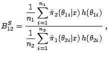
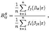
As explained in Sects. 11.2.2 and 11.2.3, the first computational difficulty associated with Bayesian testing is the derivation of the Bayes factor, of the form

$$B^{\pi}_{12} = \frac{ \displaystyle{ \int_{\Theta_1} f_1(x\vert\t... ...vert\theta_2) \pi_2(\theta_2) {\text{d}}\theta_2 } } = \frac{m_1(x)}{m_2(x)}\;,$$

where, for simplicity's sake, we have adopted the model choice perspective (that is, $\theta_1$ and $\theta_2$ may live in completely different spaces).

Specific Monte Carlo methods for the estimation of ratios of normalizing constants, or, equivalently, of Bayes factors, have been developed in the past five years. See Chen et al. (2000, Chap. 5) for a complete exposition. In particular, the importance sampling technique is rather well-adapted to the computation of those Bayes factors: Given a importance distribution, with density proportional to $g$, and a sample $\theta^{(1)},\ldots,\theta^{(T)}$ simulated from $g$, the marginal density for model  $\mathfrak{M}_i$, $m_i(x)$, is approximated by

$$\widehat{m}_i(x) = \displaystyle{ \sum_{t=1}^T f_i\left(x\vert\th... ...}^T \frac{ \pi_i\left(\theta^{(t)}\right) }{ g\left(\theta^{(t)}\right) } } \;,$$

where the denominator takes care of the (possibly) missing normalizing constants. (Notice that, if $g$ is a density, the expectation of $\pi(\theta^{(t)})/g(\theta^{(t)})$ is $1$ and the denominator should be replaced by $T$ to decrease the variance of the estimator of $m_i(x)$.) A compelling incentive, among others, for using importance sampling in the setting of model choice is that the sample $(\theta^{(1)},\ldots,\theta^{(T)})$ can be recycled for all models $\mathfrak{M}_i$ sharing the same parameters (in the sense that the models $\mathfrak{M}_i$ are parameterized in the same way, e.g. by their first moments).

Example 12 (Continuation of Example 4)   In the case the $\beta$'s are simulated from a product instrumental distribution

$$g(\beta) = \prod_{i=1}^p g_i(\beta_i)\;,$$

the sample of $\beta$'s produced for the general model of Example 2, $\mathfrak{M}_1$ say, can also be used for the restricted model, $\mathfrak{M}_2$, where $\beta_1=0$, simply by deleting the first component and keeping the following components, with the corresponding importance density being

$$g_{-1}(\beta) = \prod_{i=2}^p g_i(\beta_i)\;.$$

Once the $\beta$'s have been simulated, the Bayes factor $B^{\pi}_{12}$ can be approximated by $\widehat{m}_1(x)/\widehat{m}_2(x)$.

However, the variance of $\widehat{m}(x)$ may be infinite, depending on the choice of $g$. A possible choice is $g(\theta) = \pi(\theta)$, with wider tails than $\pi(\theta\vert x)$, but this is often inefficient if the data is informative because the prior and the posterior distributions will be quite different and most of the simulated values $\theta^{(t)}$ fall outside the modal region of the likelihood. For the choice $g(\theta) = f(x\vert\theta) \pi(\theta)$,

$$\widehat{m}(x) = 1 \bigg/\frac{1}{ T} \sum_{t=1}^T \frac{1 } { f\left(x\vert\theta^{(t)}\right)} \;,$$ (11.9)

is the harmonic mean of the likelihoods, but the corresponding variance is infinite when the likelihood has thinner tails than the prior (which is often the case). Explicitly oriented towards the computation of ratios of normalising constants, bridge sampling was introduced in [29]: if both models $\mathfrak{M}_1$ and $\mathfrak{M}_2$ cover the same parameter space $\Theta$, if $\pi_1(\theta\vert x) = c_1 {\tilde\pi}_1(\theta\vert x)$ and $\pi_2(\theta\vert x) = c_2 {\tilde\pi}_2(\theta\vert x)$, where $c_1$ and $c_2$ are unknown normalising constants, then the equality

$$\frac{c_2}{c_1} = \frac{\mathbb{E}^{\pi_2} \left[{\tilde\pi}_1(\t... ...ight]} {\mathbb{E}^{\pi_1}\left[{\tilde\pi}_2(\theta\vert x)\,h(\theta)\right]}$$

holds for any bridge function $h(\theta)$ such that both expectations are finite. The bridge sampling estimator is then

$$B^S_{12} = \frac{ \displaystyle{ \frac{1}{ n_1} \sum_{i=1}^{n_1} ... ..._2} \sum_{i=1}^{n_2} {\tilde\pi}_1(\theta_{2i}\vert x) \,h(\theta_{2i}) } } \;,$$

where the $\theta_{ji}$'s are simulated from $\pi_j(\theta\vert x)$ $(\kern.5pt j=1,2,\,i=1,\ldots,n_j)$. For instance, if

$$h(\theta) = 1/\left[ {\tilde\pi}_1(\theta\vert x) {\tilde\pi}_2(\theta_{1i}\vert x) \right]\;,$$

then $B^S_{12}$ is a ratio of harmonic means, generalizing (11.9). [29] have derived an (asymptotically) optimal bridge function

$$h^{\ast}(\theta) = \frac{n_1+n_2 }{ n_1 \pi_1(\theta\vert x) + n_2 \pi_2(\theta\vert x)}\;.$$

This choice is not of direct use, since the normalizing constants of $\pi_1(\theta\vert x)$ and $\pi_2(\theta\vert x)$ are unknown (otherwise, we should not need to resort to such techniques!). Nonetheless, it shows that a good bridge function should cover the support of both posteriors, with equal weights if $n_1=n_2$.

Example 13 (Continuation of Example 2)   For generalized linear models, the mean (conditionally on the covariates) satisfies

$$\mathbb{E}[y\vert\theta] = \nabla\psi(\theta) = \Psi\left(x^t\beta\right)\;,$$

where $\Psi$ is the link function. The choice of the link function $\Psi$ usually is quite open. For instance, when the $y$'s take values in $\{0,1\}$, three common choices of $\Psi$ are ([28])

$$\Psi_1(t) = \exp(t) / (1+\exp(t))\;,\quad \Psi_2(t) = \Phi(t)\;, \quad \Psi_3(t) = 1 - \exp(-\exp(t))\;,$$

corresponding to the logit, probit and log-log link functions (where $\Phi$ denotes the c.d.f. of the $\mathcal{N}(0,1)$ distribution). If the prior distribution $\pi$ on the $\beta$'s is a normal $\mathcal{N}_p(\xi,\tau^2 I_p)$, and if the bridge function is $h(\beta)=1/\pi(\beta)$, the bridge sampling estimate is then $(1\le i<j\le 3)$

$$B^S_{ij} = \frac{ \displaystyle{ \frac{1}{ n} \sum_{t=1}^{n} f_j(... ...) } }{ \displaystyle{ \frac{1}{ n} \sum_{t=1}^{n} f_i(\beta_{jt}\vert x) } }\;,$$

where the $\beta_{it}$ are generated from $\pi_i(\beta_i\vert x)\propto f_i(\beta_i\vert x)\pi(\beta_i)$, that is, from the true posteriors for each link function.

As can be seen from the previous developments, such methods require a rather careful tuning to be of any use. Therefore, they are rather difficult to employ outside settings where pairs of models are opposed. In other words, they cannot be directly used in general model choice settings where the parameter space (and in particular the parameter dimension) varies across models, like, for instance, Example 7. To address the computational issues corresponding to these cases requires more advanced techniques introduced in the next section.