18.2 Projection Pursuit

``Projection Pursuit'' stands for a class of exploratory projection techniques. This class contains statistical methods designed for analyzing high-dimensional data using low-dimensional projections. The aim of projection pursuit is to reveal possible nonlinear and therefore interesting structures hidden in the high-dimensional data. To what extent these structures are ``interesting'' is measured by an index. Exploratory Projection Pursuit (EPP) goes back to Kruskal(1972,1969). The approach was successfully implemented for exploratory purposes by various other authors. The idea has been applied to regression analysis, density estimation, classification and discriminant analysis.

Exploratory Projection Pursuit

In EPP, we try to find ``interesting'' low-dimensional projections of the data. For this purpose, a suitable index function $I(\alpha)$, depending on a normalized projection vector $\alpha$, is used. This function will be defined such that ``interesting'' views correspond to local and global maxima of the function. This approach naturally accompanies the technique of principal component analysis (PCA) of the covariance structure of a random vector $X$. In PCA we are interested in finding the axes of the covariance ellipsoid. The index function $I(\alpha)$ is in this case the variance of a linear combination $\alpha^{\top} X$ subject to the normalizing constraint $\alpha^{\top} \alpha=1$ (see Theorem 9.2). If we analyze a sample with a $p$-dimensional normal distribution, the ``interesting'' high-dimensional structure we find by maximizing this index is of course linear.

There are many possible projection indices, for simplicity the kernel based and polynomial based indices are reported. Assume that the $p$-dimensional random variable $X$ is sphered and centered, that is, $E(X)=0$ and $\Var(X) = {\cal{I}}_p$. This will remove the effect of location, scale, and correlation structure. This covariance structure can be achieved easily by the Mahalanobis transformation (3.26).

Friedman and Tukey (1974) proposed to investigate the high-dimensional distribution of $X$ by considering the index

$$I_{\textrm{FT},h}(\alpha) = n^{-1}\sum_{i=1}^n\hat{f}_{h,\alpha}(\alpha^{\top}X_i)$$ (18.5)

where $\hat{f}_{h,\alpha}$ denotes the kernel estimator (see Section 1.3)

$$\hat{f}_{h,\alpha}(z) = n^{-1}\sum_{j=1}^nK_h(z-\alpha^{\top}X_j)$$ (18.6)

of the projected data. Note that (18.5) is an estimate of $\int f^2(z) dz$ where $z=\alpha^{\top}X$ is a one-dimensional random variable with mean zero and unit variance. If the high-dimensional distribution of $X$ is normal, then each projection $z=\alpha^{\top}X$ is standard normal since $\vert\vert\alpha\vert\vert=1$ and since $X$ has been centered and sphered by, e.g., the Mahalanobis transformation.

The index should therefore be stable as a function of $\alpha$ if the high-dimensional data is in fact normal. Changes in $I_{\textrm{FT},h}(\alpha)$ with respect to $\alpha$ therefore indicate deviations from normality. Hodges and Lehman (1956) showed that, given a mean of zero and unit variance, the (compact support) density which minimizes $\int f^2$ is uniquely given by

$$f(z)=\max\{0,c (b^2-z^2)\},$$

where $c=3/(20\sqrt{5})$ and $b=\sqrt{5}$. This is a parabolic density function, which is equal to zero outside the interval ( $-\sqrt{5},\sqrt{5}$). A high value of the Friedman-Tukey index indicates a larger departure from the parabolic form.

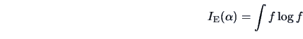
An alternative index is based on the negative of the entropy measure, i.e., $\int -f \log f$. The density for zero mean and unit variance which minimizes the index

$$\int f \log f$$

is the standard normal density, a far more plausible candidate than the parabolic density as a norm from which departure is to be regarded as ``interesting''. Thus in using $\int f \log f$ as a projection index we are really implementing the viewpoint of seeing ``interesting'' projections as departures from normality. Yet another index could be based on the Fisher information (see Section 6.2)

$$\int (f')^2/f.$$

To optimize the entropy index, it is necessary to recalculate it at each step of the numerical procedure. There is no method of obtaining the index via summary statistics of the multivariate data set, so the workload of the calculation at each iteration is determined by the number of observations. It is therefore interesting to look for approximations to the entropy index. Jones and Sibson (1987) suggested that deviations from the normal density should be considered as

$$f(x)=\varphi (x)\{1+\varepsilon(x)\}$$ (18.7)

where the function $\varepsilon$ satisfies

$$\int \varphi (u) \varepsilon (u)u^{-r} du=0,\textrm{ for } r=0,1,2.$$ (18.8)

In order to develop the Jones and Sibson index it is convenient to think in terms of cumulants $\kappa_3=\mu_3=E(X^3)$, $\kappa_4=\mu_4=E(X^4)-3$ (see Section 4.2). The standard normal density satisfies $\kappa_3=\kappa_4=0$, an index with any hope of tracking the entropy index must at least incorporate information up to the level of symmetric departures ($\kappa_3$ or $\kappa_4$ not zero) from normality. The simplest of such indices is a positive definite quadratic form in $\kappa_3$ and $\kappa_4$. It must be invariant under sign-reversal of the data since both $\alpha^{\top} X$ and $-\alpha^{\top}X$ should show the same kind of departure from normality. Note that $\kappa_3$ is odd under sign-reversal, i.e., $\kappa_3(\alpha^{\top}X)=-\kappa_3(-\alpha^{\top}X)$. The cumulant $\kappa_4$ is even under sign-reversal, i.e., $\kappa_4(\alpha^{\top}X)=\kappa_4(-\alpha^{\top}X)$. The quadratic form in $\kappa_3$ and $\kappa_4$ measuring departure from normality cannot include a mixed $\kappa_3 \kappa_4$ term.

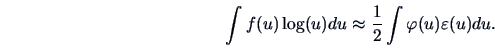
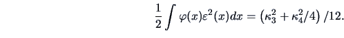
For the density (18.7) one may conclude with (18.8) that

$$\int f(u)\log(u)du\approx\frac{1}{2}\int \varphi (u)\varepsilon(u)du.$$

Now if $f$ is expressed as a Gram-Charliér expansion

$$f(x)\varphi(x)=\{1+\kappa_3H_3(x)/6+\kappa_4H_4(x)/24...\}$$ (18.9)

(Kendall and Stuart; 1977, p. 169) where $H_r$ is the $r$-th Hermite polynomial, then the truncation of (18.9) and use of orthogonality and normalization properties of Hermite polynomials with respect to $\varphi$ yields

$$\frac{1}{2}\int \varphi (x)\varepsilon^2 (x)dx=\left(\kappa_3^2+\kappa_4^2 /4\right)/12.$$

The index proposed by Jones and Sibson (1987) is therefore

$$I_{JS}(\alpha)=\{\kappa_3^2 (\alpha^{\top}X)+\kappa_4^2 (\alpha^{\top}X)/4\}/12.$$

This index measures in fact the difference $\int f \log f - \int\varphi\log\varphi$.

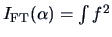
EXAMPLE 18.1   The exploratory Projection Pursuit is used on the Swiss bank note data. For 50 randomly chosen one-dimensional projections of this six-dimensional dataset we calculate the Friedman-Tukey index to evaluate how ``interesting'' their structures are.

Figure: Exploratory Projection Pursuit for the Swiss bank notes data (green = standard normal, red = best, blue = worst). MVAppexample.xpl

Figure 18.3 shows the density for the standard, normally distributed data (green) and the estimated densities for the best (red) and the worst (blue) projections found. A dotplot of the projections is also presented. In the lower part of the figure we see the estimated value of the Friedman-Tukey index for each computed projection. From this information we can judge the non normality of the bank note data set since there is a lot of variation across the 50 random projections.

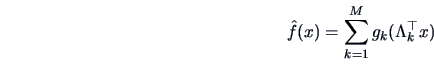
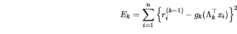
Projection Pursuit Regression

The problem in projection pursuit regression is to estimate a response surface

$$f(x) = E(Y\mid x)$$

via approximating functions of the form

$$\hat{f}(x) = \sum_{k=1}^{M} g_k(\Lambda_k^{\top} x)$$

with non-parametric regression functions $g_k$. Given observations $\{(x_1,y_1), ..., (x_n,y_n)\}$ with $x_i \in {\mathbb{R}}^p$ and $y_i \in {\mathbb{R}}$ the basic algorithm works as follows.

1. Set $r_i^{(0)} = y_i$ and $k=1$.
2. Minimize
   
   $$E_k = \sum_{i=1}^{n} \left\{r_i^{(k-1)} - g_k (\Lambda_k^{\top} x_i)\right\}^2$$
   
   
   where $\Lambda_k$ is an orthogonal projection matrix and $g_k$ is a non-parametric regression estimator.
3. Compute new residuals
   
   $$r_i^{(k)} = r_i^{(k-1)} - g_k(\Lambda_k^{\top} x_i).$$
   
   

4. Increase $k$ and repeat the last two steps until $E_k$ becomes small.

Although this approach seems to be simple, we encounter some problems. One of the most serious is that the decomposition of a function into sums of functions of projections may not be unique. An example is

$$z_1 z_2 = \frac{1}{4ab} \{(a z_1 + b z_2)^2 - (a z_1 - b z_2)^2 \}.$$

Improvements of this algorithm were suggested by Friedman and Stuetzle (1981).

Summary

$\ast$

Exploratory Projection Pursuit is a technique used to find interesting structures in high-dimensional data via low-dimensional projections. Since the Gaussian distribution represents a standard situation, we define the Gaussian distribution as the most uninteresting.

$\ast$

The search for interesting structures is done via a projection score like the Friedman-Tukey index $I_{\textrm{FT}}(\alpha)=\int f^2$. The parabolic distribution has the minimal score. We maximize this score over all projections.

$\ast$

The Jones-Sibson index maximizes

$$I_{\textrm{JS}}(\alpha)=\{\kappa_3(\alpha^{\top}X)+\kappa_4^2(\alpha^{\top}X)/4\}/12$$

as a function of $\alpha$.

$\ast$

The entropy index maximizes

$$I_{\textrm{E}}(\alpha)=\int f\log f$$

where $f$ is the density of $\alpha^{\top} X$.

$\ast$

In Projection Pursuit Regression the idea is to represent the unknown function by a sum of non-parametric regression functions on projections. The key problem is in choosing the number of terms and often the interpretability.